When working with audio plug-ins, you may stumble upon the term “transfer function” – for example our latest plug-in smart:comp 2 sports a new feature called “free-form transfer function”. In this article we want to outline the concept of transfer functions in general, explain why transfer functions are particularly interesting when trying to understand the behavior of a compressor and how a freely adjustable transfer function can open up a lot of creative possibilities.
Before heading into the details of compressor transfer functions, let’s take a look at their basic concept. In engineering, a so-called transfer function is a mathematical way to model the output of a system for each possible input. When looking at a 2-dimensional transfer function graph, the horizontal axis (x-axis) represents all possible input values and the vertical axis (y-axis) represents the corresponding output values. So, the function describes how an input is transferred to a certain output value.
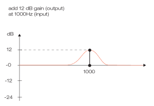
A well-known and quite intuitive example for a transfer function in audio production is the graphic equalizer: The x-axis represents all frequencies while the y-axis represents the gain at a specific frequency. Hence, the EQ curve describes the output value (gain) at a certain input (frequency).
Another widely used but a little trickier transfer function is the so-called compressor graph (also known as compressor curve or compressor transfer function). In this case, the transfer function represents a direct mapping from an input level (x-axis) to an output level (y-axis).
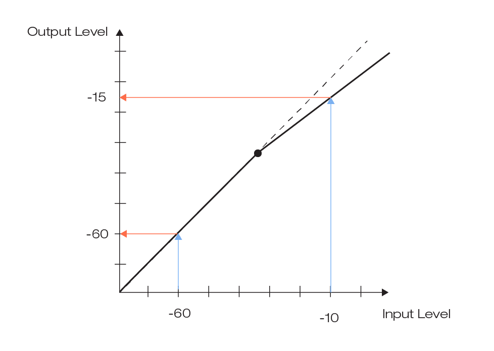
As you may already know, a typical compressor graph is a diagonal line below a threshold value that becomes flatter above the threshold (if the signal is being compressed). This tells us that input values below the threshold are mapped to the exact same output values, while input values above the threshold are mapped to smaller output values – they are compressed.
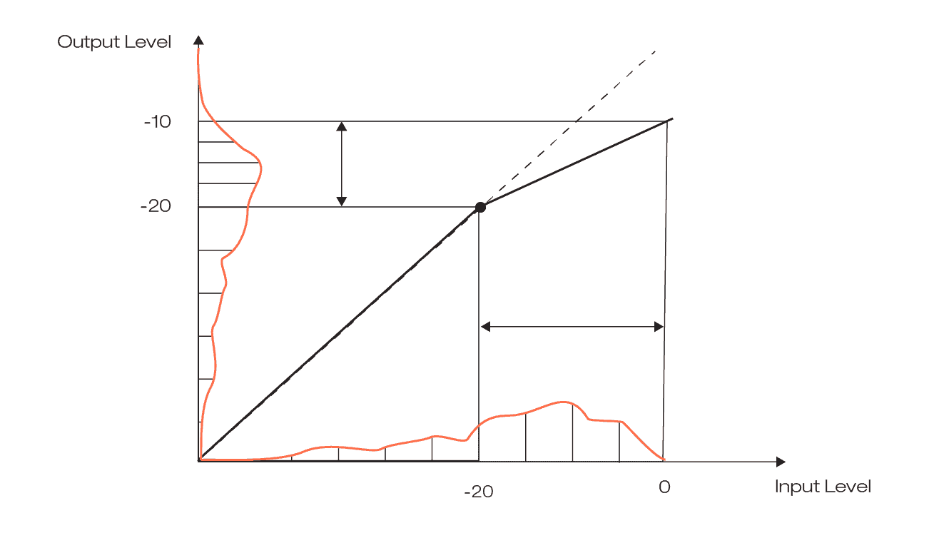
The impact of this kind of classical compression becomes quite obvious when looking at the average level distribution (called level histogram) of a signal before and after compression. Since the distribution shows how often a certain level is observed in a signal, a broad distribution indicates a lot of different signal levels (high dynamics), while a narrow distribution indicates only small level variations and low dynamics.
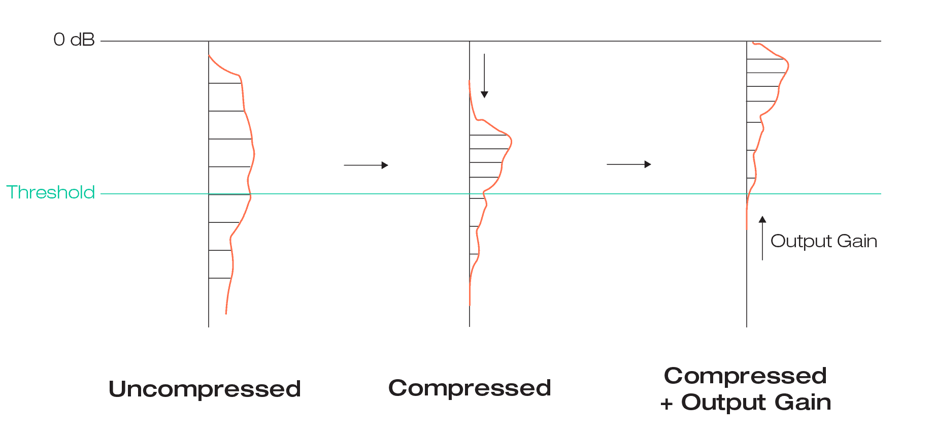
By adding makeup gain to the compressed signal, the average signal level can be moved up to its original range – this combination of peak compression plus make-up gain is called downward compression.
This is what’s happening to a level histogram when going through this process: by applying compression, the distribution above the threshold becomes narrower as the levels are squeezed closer together, while the distribution below the threshold remains more or less unchanged. That’s expected, since that’s the typical application for a compressor: reducing dynamics. By adding a makeup-gain, the histogram is moved back to the level of the original histogram, but it is narrower now.
What happens if the transfer function below the threshold is no longer a straight line? It means that any input level can be mapped to any output level. A typical and simple example for this kind of mapping is a gate: all input values below the lower threshold are mapped to an output value of zero. As a consequence, all signal levels below the threshold vanish in the output signal.
smart:comp 2 allows you to go even further by offering a free-form transfer function. That means that quite complex mappings from input to output can be achieved. Why is that so tempting? Let’s look at three different examples:
You may already have heard the term “parallel compression”. What this compression technique typically tries to achieve is boosting low-level components by mixing a heavily compressed version and an uncompressed (or almost uncompressed) version of a signal. Rather than lowering the highest peaks as known from downward compression, this technique decreases the dynamic range by raising up low signal levels.
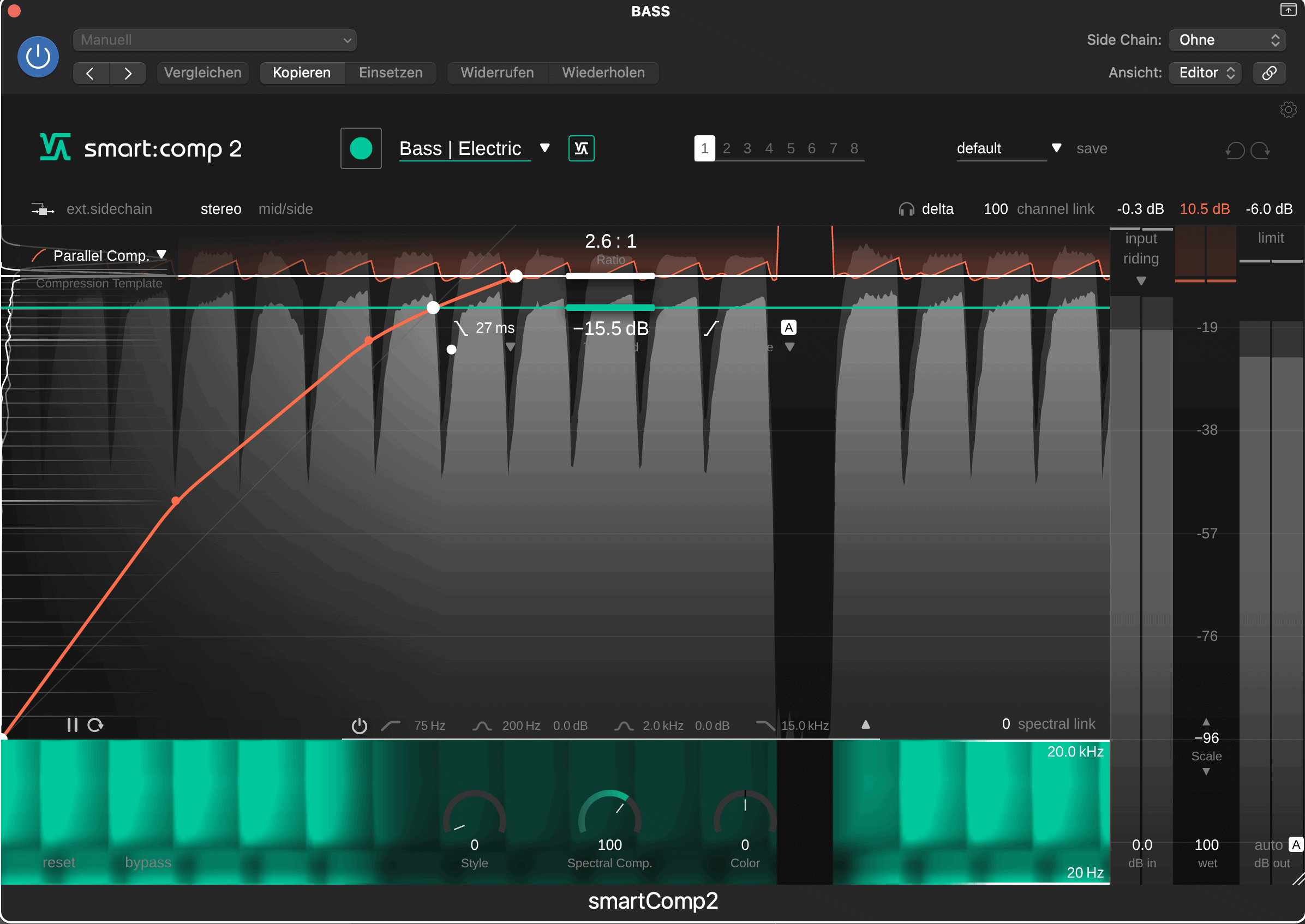
Upward compression can be great way to generate a very dense and compact sound, since transients are retained (no downward compression) while the dynamics of the signal are still reduced.
With smart:comp 2’s free-form transfer function it’s extremely easy to achieve this effect by simply increasing the output level for low input signal with an additional control point or by selecting the respective transfer function template.
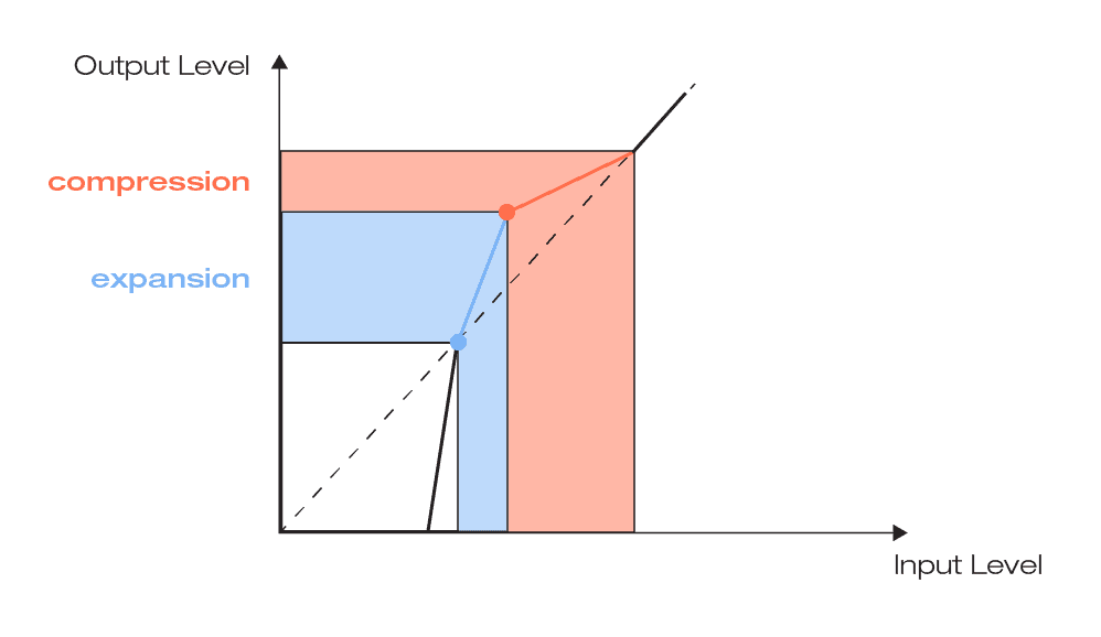
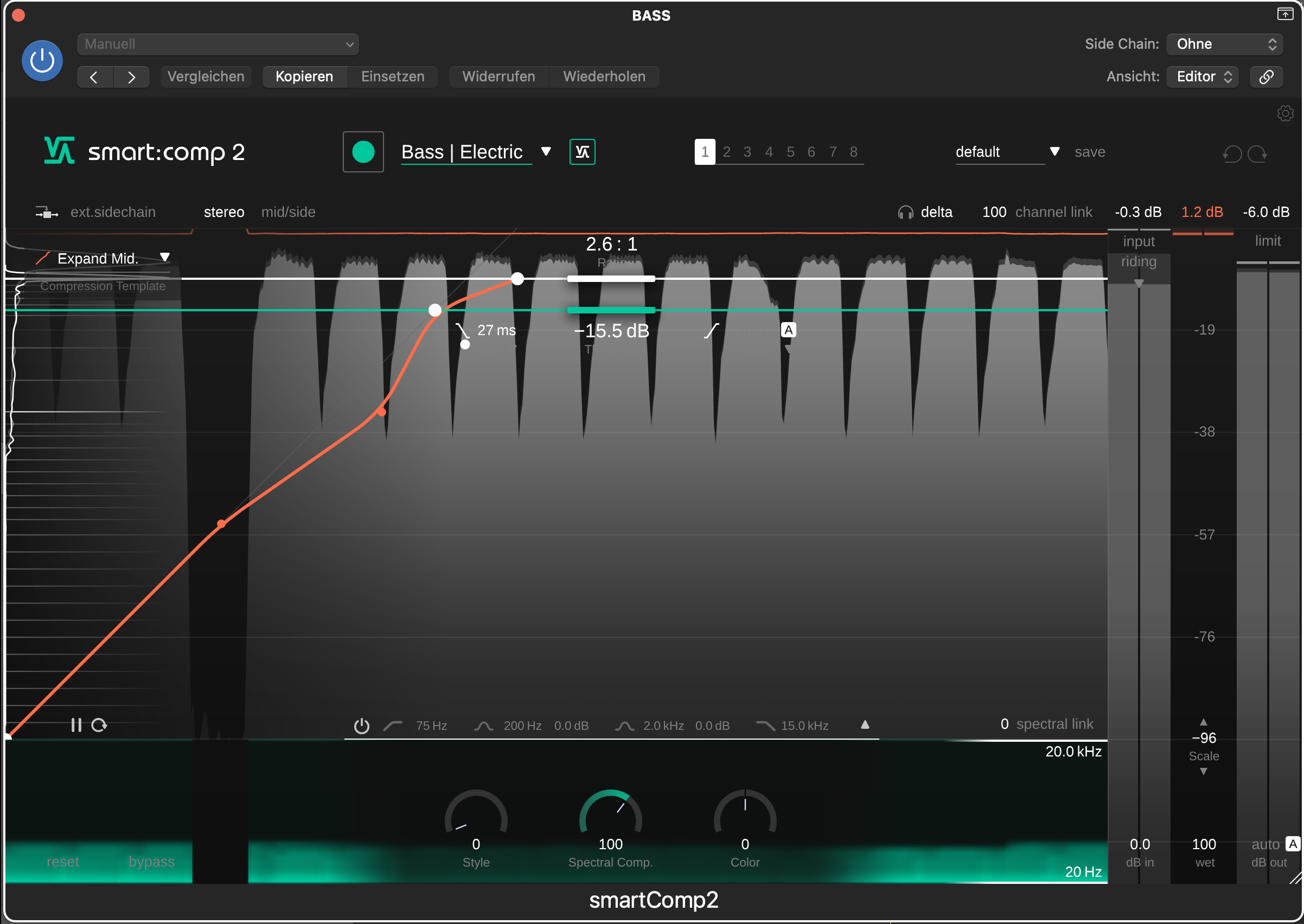
Typically, most of the energy of a signal lies around the average signal level. Mid-level expansion is a great way to increase the dynamics around this average signal range while compressing the peaks. That way, you can keep the overall dynamics more or less untouched, but you can shift the dynamic focus to the mid-range.
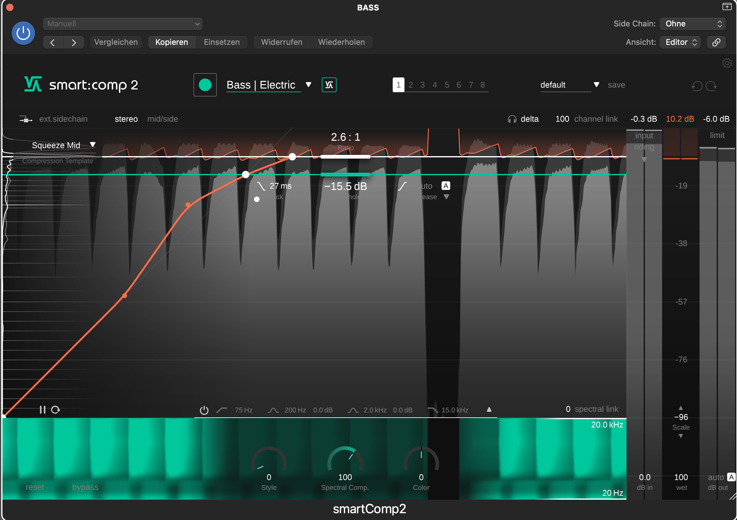
The opposite of mid-level expansion is mid-level compression. By compressing the mid-range, you can create a compact sound without having to tame transient peaks. This technique helps to let the transients of a signal stand out while giving your track a nice dense character.
These are just three examples of what’s possible with smart:comp 2’s free-form transfer function. Obviously, you can also apply more unique mappings and go for interesting creative effects or a very specific compression character.
Want to get creative? Get inspired and check out the 30 day free demo of smart:comp 2 here.